Plot a Least Squares Regression Line

CODAP makes it possible to plot a least squares regression line on a graph that has numerical attributes on both the horizontal axis (X axis) and the vertical axis (Y axis). To add a least squares regression line to a graph, go to the inspector palette to the right of the graph, click on the ruler icon, and select “Least Squares Line” (if you do not see an option for “Least Squares Line,” CODAP may be treating one or both of your attributes as categorical–to fix this, click on the name of the attribute on the graph and select “Treat as Numeric”).

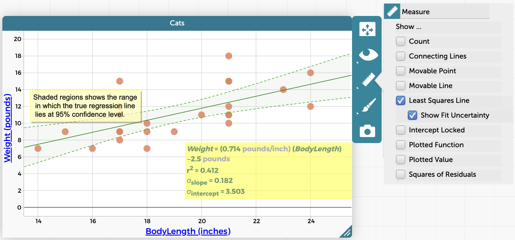
After selecting the check box for “Least Squares Line,” the least squares line will appear, as will a yellow box showing the formula used to calculate the line as well as the value of the R2 coefficient of determination. Note that this yellow box can be dragged around the graph to a new position, which is useful to do if you do not want to cover up points on the graph. As shown in the image below, you may also select “Show Fit Uncertainty,” which adds a 95% confidence range to the least squares line and also adds the values of the standard error (σ) of the slope and the intercept to the yellow box on the graph with the regression equation and R2 value. Mousing over the shaded region makes the second yellow box appear describing the 95% confidence level.

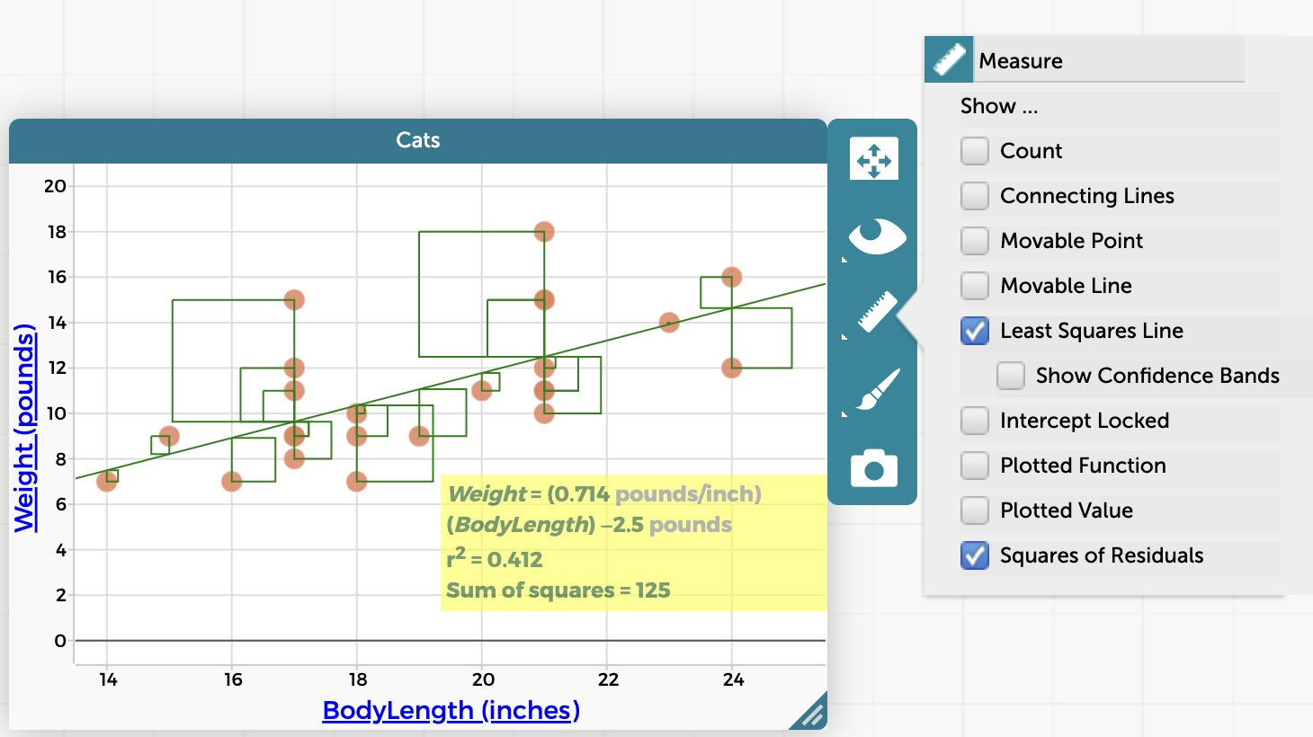
Also, try selecting “Squares of Residuals” from the ruler/measure menu–this will give you visual representations of the square of the distance of each point from the least squares line (see image below). Adding the squares of residuals to the graph will also add the sum of squares value to the yellow box on the graph.

Note that it is also possible to manually simulate linear regression by plotting a movable line, adding the squares of residuals from the Measure/ruler menu, and dragging the line around to find the best fit to the data, minimizing the value of the sum of squares.